Non-simulation based likelihood model diagnostic

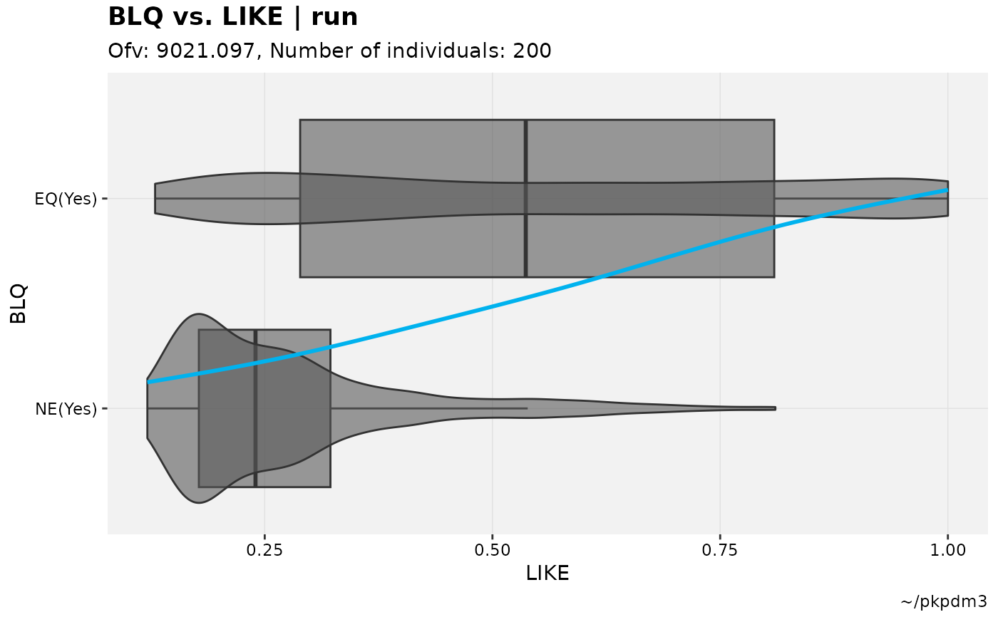
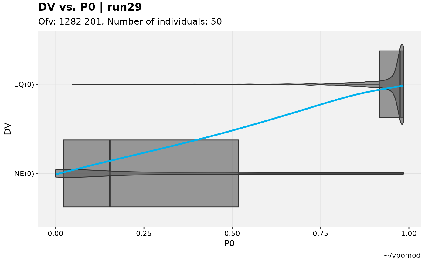
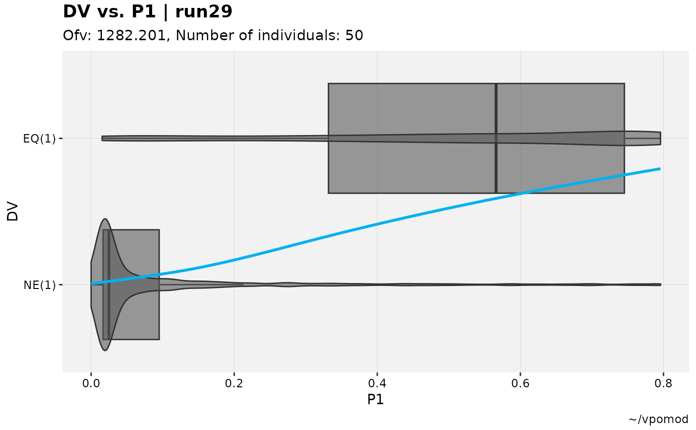
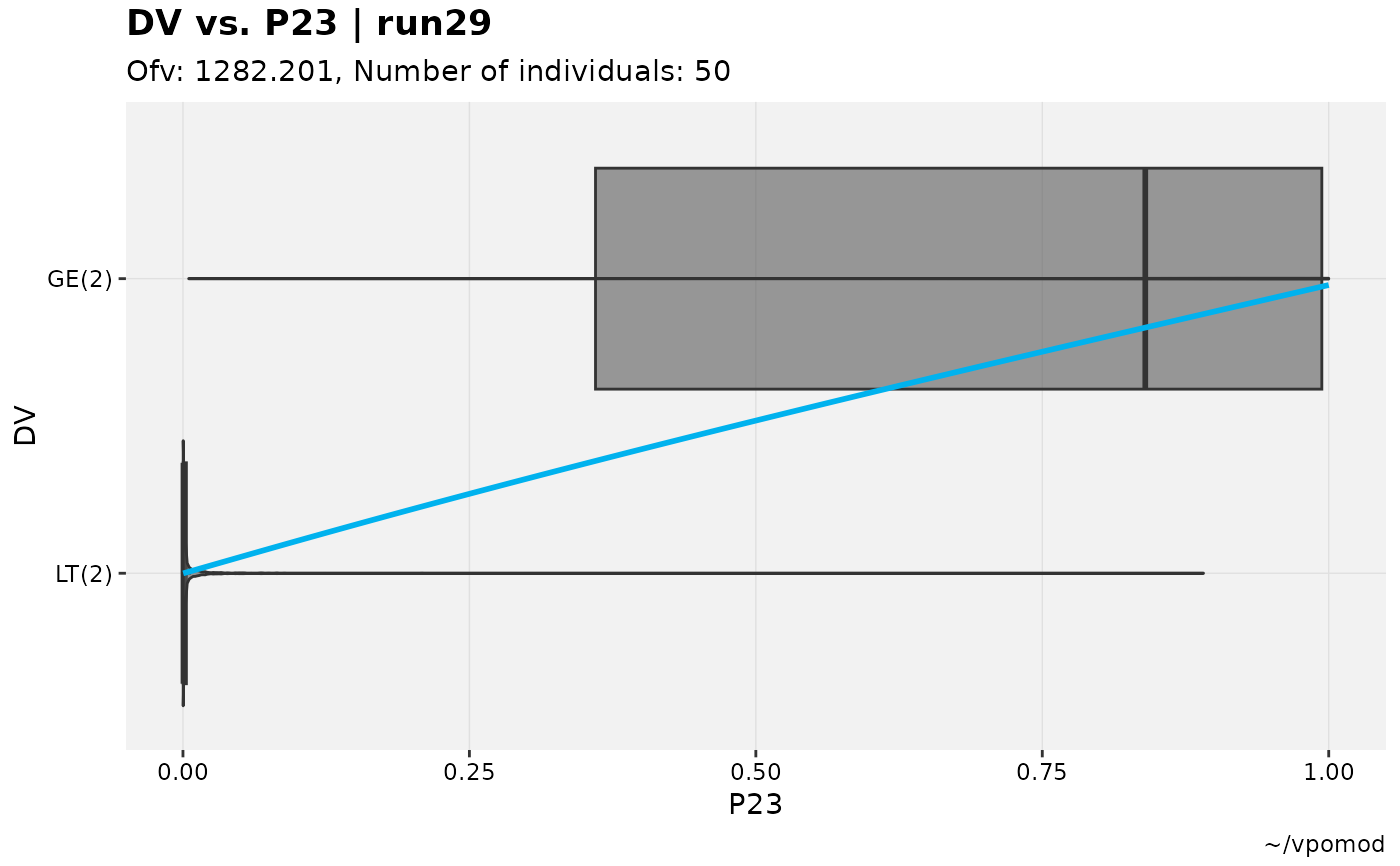
These plots attempt to provide a means of verifying that the estimated likelihoods and probabilities for categorical outcomes are captured within the model.

When the smooth spline is included (type includes "s"), it is expected that the overall trend is up and to the right; a relatively flat trend suggests that the modeled likelihood is inconsistent with the observed outcome.

Usage

catdv_vs_dvprobs(
  xpdb,
  mapping = NULL,
  cutpoint = 1,
  type = "vbs",
  title = "@y vs. @x | @run",
  subtitle = "Ofv: @ofv, Number of individuals: @nind",
  caption = "@dir",
  tag = NULL,
  xlab = c("probability", "basic"),
  facets,
  .problem,
  quiet,
  ...
)

Arguments

xpdb

<xp_xtras> or <xpose_data> object

mapping

ggplot2 style mapping

cutpoint

<numeric> Of defined probabilities, which one to use in plots.

type

See Details.

title

Plot title

subtitle

Plot subtitle

caption

Plot caption

tag

Plot tag

xlab

Either use the typical basic x-axis label (the cutpoint-defined column name) or label it based on the probability/likelihood it is estimating.

facets

Additional facets

.problem

Problem number

quiet

Silence extra debugging output

...

Any additional aesthetics.

Value

The desired plot

Examples

# Test M3 model
pkpd_m3 %>%
  # Need to ensure var types are set
  set_var_types(catdv=BLQ,dvprobs=LIKE) %>%
  # Set probs
  set_dv_probs(1, 1~LIKE, .dv_var = BLQ) %>%
  # Optional, but useful to set levels
  set_var_levels(1, BLQ = lvl_bin()) %>%
  # Plot with basic xlab makes no assumptions
  catdv_vs_dvprobs(xlab = "basic")
#> Using data from $prob no.1
#> Filtering data by EVID == 0
#> `geom_smooth()` using method = 'gam' and formula = 'y ~ s(x, bs = "cs")'
#> `geom_smooth()` using method = 'gam' and formula = 'y ~ s(x, bs = "cs")'


# Test categorical model
vismo_xpdb <- vismo_pomod  %>%
  set_var_types(.problem=1, catdv=DV, dvprobs=matches("^P\\d+$")) %>%
  set_dv_probs(.problem=1, 0~P0,1~P1,ge(2)~P23)

# Various cutpoints (note axes labels and texts)
vismo_xpdb %>%
  catdv_vs_dvprobs(xlab = "basic")
#> Using data from $prob no.1
#> Filtering data by EVID == 0
#> `geom_smooth()` using method = 'gam' and formula = 'y ~ s(x, bs = "cs")'
#> `geom_smooth()` using method = 'gam' and formula = 'y ~ s(x, bs = "cs")'

vismo_xpdb %>%
  catdv_vs_dvprobs(cutpoint = 2, xlab = "basic")
#> Using data from $prob no.1
#> Filtering data by EVID == 0
#> `geom_smooth()` using method = 'gam' and formula = 'y ~ s(x, bs = "cs")'
#> `geom_smooth()` using method = 'gam' and formula = 'y ~ s(x, bs = "cs")'

vismo_xpdb %>%
  catdv_vs_dvprobs(cutpoint = 3, xlab = "basic")
#> Using data from $prob no.1
#> Filtering data by EVID == 0
#> `geom_smooth()` using method = 'gam' and formula = 'y ~ s(x, bs = "cs")'
#> `geom_smooth()` using method = 'gam' and formula = 'y ~ s(x, bs = "cs")'


# Latter is arguably clearer with default xlab
vismo_xpdb %>%
  catdv_vs_dvprobs(cutpoint = 3)
#> Using data from $prob no.1
#> Filtering data by EVID == 0
#> `geom_smooth()` using method = 'gam' and formula = 'y ~ s(x, bs = "cs")'
#> `geom_smooth()` using method = 'gam' and formula = 'y ~ s(x, bs = "cs")'