The extended xpose data object • xpose.xtras

How to get the object

The xpose_data object (aka: xpdb) gets a few extensions in this package. Many of these are added to accommodate new plots and features, but in most cases these features are cross-compatible with a typical xpose_data object as well. The extended version of xpose_data has the class xp_xtra, and is also referred to as xpdb_x.

Conversion of an xpose_data object is simple.

xpdb_converted <- xpdb_ex_pk %>%
  as_xpdb_x()

# To verify:
xpdb_ex_pk
#> run001.lst overview: 
#>  - Software: nonmem 7.3.0 
#>  - Attached files (memory usage 1.4 Mb): 
#>    + obs tabs: $prob no.1: catab001.csv, cotab001, patab001, sdtab001 
#>    + sim tabs: $prob no.2: simtab001.zip 
#>    + output files: run001.cor, run001.cov, run001.ext, run001.grd, run001.phi, run001.shk 
#>    + special: <none> 
#>  - gg_theme: theme_readable 
#>  - xp_theme: theme_xp_default 
#>  - Options: dir = data, quiet = FALSE, manual_import = NULL
xpdb_converted
#> 
#> ── ~ xp_xtras object 
#> Model description: NONMEM PK example for xpose
#> run001.lst overview: 
#>  - Software: nonmem 7.3.0 
#>  - Attached files (memory usage 1.4 Mb): 
#>    + obs tabs: $prob no.1: catab001.csv, cotab001, patab001, sdtab001 
#>    + sim tabs: $prob no.2: simtab001.zip 
#>    + output files: run001.cor, run001.cov, run001.ext, run001.grd, run001.phi, run001.shk 
#>    + special: <none> 
#>  - gg_theme: theme_readable 
#>  - xp_theme: xp_xtra_theme new_x$xp_theme 
#>  - Options: dir = data, quiet = FALSE, manual_import = NULL, cvtype = exact

As shown, there are some minor changes to the output for print() to help confirm if an object is the extended version. However, this is implemented merely as an S3 class, so all xpose functions will continue to work with this new object; the current package is also written in a way to work even if the xp_xtra object loses that class.

Notably, there is no convenience function to read a model output directly to an xp_xtra object, so all objects labelled as xp_xtra start as xpose_data.

Many example xp_xtra objects are included in this package, covering a variety of special cases.

What features are available?

Tidying up

It is by design that xpose attempts to align well with the tidyverse family of R packages, so one focus of the extension package is to make that alignment a bit more consistent. For example, xpose::set_var_types accepts character vectors of column names, but not tidyselection. As such, columns named in a consistent and tidyselect-friendly way cannot be used to an advantage. A minimal example can be seen below, but of course there are more complex situations where this is convenient.

# Unset all example covariates
xpdb_ex_covs <- xp_var(xpdb_ex_pk, type = c("catcov","contcov"), .problem=1) %>% 
  pull(col)
xpdb_ex_covs
#> [1] "MED1" "MED2" "SEX"  "AGE"  "CLCR" "WT"
no_covs <- set_var_types(xpdb_ex_pk, .problem=1, na = xpdb_ex_covs)

# set_var_types on xpose_data objects uses xpose::set_var_types
set_var_types(no_covs, .problem=1, catcov = c("MED1","MED2")) %>%
  xp_var(type = c("catcov","contcov"), .problem=1) %>% 
  pull(col)
#> [1] "MED1" "MED2"
no_covs %>%
  as_xpdb_x() %>%
  set_var_types(catcov = starts_with("MED"), .problem=1) %>%
  xp_var(type = c("catcov","contcov"), .problem=1) %>% 
  pull(col)
#> [1] "MED1" "MED2"

Tidyselection is used fairly heavily in the xpose.xtras package where it seems intuitive to include it. There are likely functions that could use it but do not currently. As such, the documentation does attempt to distinguish where tidyselect is expected.

Labels, units and (also) levels

Another feature includes a few visual confirmations of variable units, labels and (new to this package) levels. In xpose, users are able to add units and labels to any variable, which are stored in the object and are theoretically used somewhere. This package attempts to use these communication features more liberally in plots and for the user, but broader implementation (some of which require changes to existing xpose functions) is not complete just yet.

With labels and units, these are applied using the conventional xpose functions. However, unlike in xpose, these can be confirmed using list_vars() in xpose.xtras.

w_unit_labs <- xpdb_x %>%
  set_var_labels(AGE="Age", MED1 = "Digoxin", .problem = 1) %>%
  set_var_units(AGE="yrs")
list_vars(w_unit_labs, .problem = 1)
#> List of available variables for problem no. 1
#>  - Subject identifier (id)               : ID
#>  - Dependent variable (dv)               : DV
#>  - Independent variable (idv)            : TIME
#>  - Dose amount (amt)                     : AMT
#>  - Event identifier (evid)               : EVID
#>  - Model typical predictions (pred)      : PRED
#>  - Model individual predictions (ipred)  : IPRED
#>  - Model parameter (param)               : KA, CL, V, ALAG1
#>  - Eta (eta)                             : ETA1, ETA2, ETA3
#>  - Residuals (res)                       : CWRES, IWRES, RES, WRES
#>  - Categorical covariates (catcov)       : SEX [0], MED1 ('Digoxin') [0], MED2 [0]
#>  - Continuous covariates (contcov)       : CLCR, AGE ('Age', yrs), WT
#>  - Compartment amounts (a)               : A1, A2
#>  - Not attributed (na)                   : DOSE, SS, II, TAD, CPRED

Levels can also be added to any variable, but can be especially useful for categorical covariates (catcov) and categorical DVs (type catdv, added by this package). The documentation for set_var_levels() can be referenced for more information about this, but the example below shows how this feature can be used and checked.

w_levels <- w_unit_labs  %>%
  set_var_levels(SEX=lvl_sex(), MED1 = lvl_bin())
list_vars(w_levels, .problem = 1)
#> List of available variables for problem no. 1
#>  - Subject identifier (id)               : ID
#>  - Dependent variable (dv)               : DV
#>  - Independent variable (idv)            : TIME
#>  - Dose amount (amt)                     : AMT
#>  - Event identifier (evid)               : EVID
#>  - Model typical predictions (pred)      : PRED
#>  - Model individual predictions (ipred)  : IPRED
#>  - Model parameter (param)               : KA, CL, V, ALAG1
#>  - Eta (eta)                             : ETA1, ETA2, ETA3
#>  - Residuals (res)                       : CWRES, IWRES, RES, WRES
#>  - Categorical covariates (catcov)       : SEX [2], MED1 ('Digoxin') [2], MED2 [0]
#>  - Continuous covariates (contcov)       : CLCR, AGE ('Age', yrs), WT
#>  - Compartment amounts (a)               : A1, A2
#>  - Not attributed (na)                   : DOSE, SS, II, TAD, CPRED

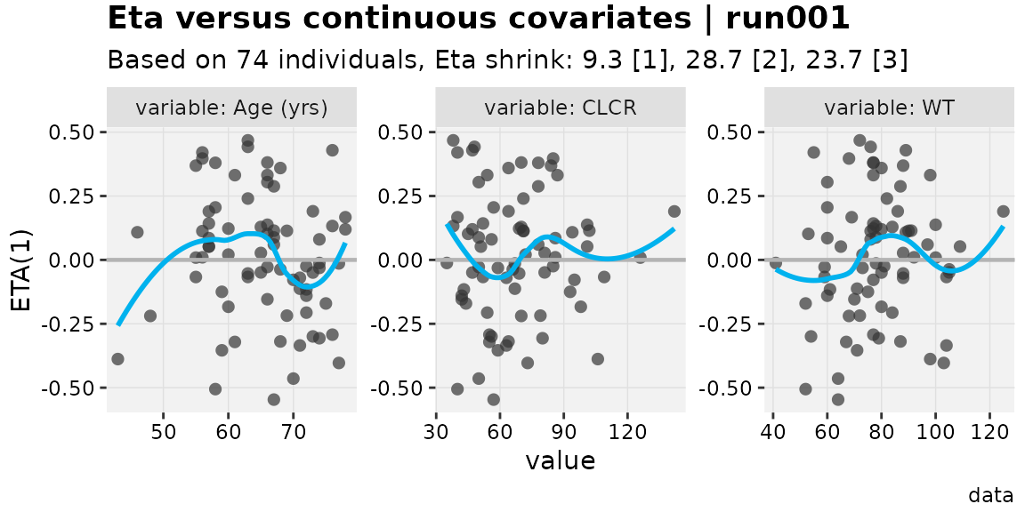
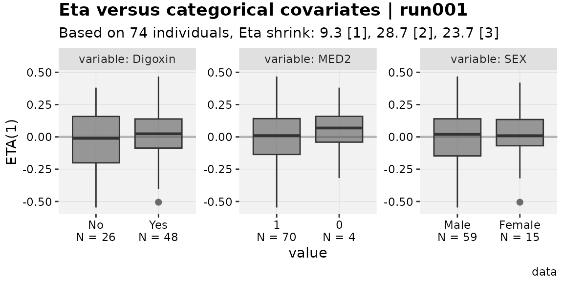
Labels, units and levels also appear in new plotting functions. There are some more complex functions where this renaming has not been implemented, but the plan is to have it be universal eventually.

eta_vs_contcov(w_unit_labs,etavar=ETA1, quiet=TRUE)
#> `geom_smooth()` using formula = 'y ~ x'
#> `geom_smooth()` using formula = 'y ~ x'

eta_vs_catcov(w_levels,etavar=ETA1, quiet=TRUE)

Note in the categorical plots, the number of individuals represented by each category is underneath the value. This is similar to the presentation in the package pmplots, but uses the existing xpose framework. This option requires the use of an xp_xtra object, and can be disabled with the argument show_n=FALSE.

Parameter tables

The get_prm() function in xpose has been extended to output coefficient of variation percent (CV%) for $\omega^2$ parameters and shrinkages where relevant.

get_prm(pheno_final) %>%
  select(-c(fixed,m,n))
#> Returning parameter estimates from $prob no.1, subprob no.1, method foce
#> # A tibble: 7 × 9
#>   type  name       label       value         se      rse diagonal      cv    shk
#>   <chr> <chr>      <chr>     <num:4>    <num:4>  <num:4> <lgl>    <num:4> <num:>
#> 1 the   THETA1     "CLpkg"  0.004813  0.0002365  0.04914 NA         NA      NA  
#> 2 the   THETA2     "Vpkg"   0.9964    0.02642    0.02652 NA         NA      NA  
#> 3 the   THETA3     "RUVADD" 2.784     0.2513     0.09027 NA         NA      NA  
#> 4 ome   OMEGA(1,1) "IIVCL"  0.2009    0.05108    0.2543  TRUE       20.30   20.1
#> 5 ome   OMEGA(2,1) ""       0.7236    0.2654     0.3668  FALSE      NA      NA  
#> 6 ome   OMEGA(2,2) "IIVV"   0.1576    0.02614    0.1659  TRUE       15.86   11.6
#> 7 sig   SIGMA(1,1) ""       1        NA         NA       TRUE       NA      19.6

There are a few options to change CV% where an opinion might conflict with the default. One such option is to add a description of how the parameter is used, which results in an exact CV% determined through integration to be used. For example, if variability on the weight-normalized clearance and volume of distribution parameters in one of the example models was logit-normally distributed, it could be described as follows.

pheno_final %>%
   add_prm_association(CLpkg~logit(IIVCL),Vpkg~logit(IIVV)) %>%
   get_prm() %>%
  select(-c(fixed,m,n))
#> Returning parameter estimates from $prob no.1, subprob no.1, method foce
#> # A tibble: 7 × 9
#>   type  name       label       value         se      rse diagonal       cv   shk
#>   <chr> <chr>      <chr>     <num:4>    <num:4>  <num:4> <lgl>     <num:4> <num>
#> 1 the   THETA1     "CLpkg"  0.004813  0.0002365  0.04914 NA       NA        NA  
#> 2 the   THETA2     "Vpkg"   0.9964    0.02642    0.02652 NA       NA        NA  
#> 3 the   THETA3     "RUVADD" 2.784     0.2513     0.09027 NA       NA        NA  
#> 4 ome   OMEGA(1,1) "IIVCL"  0.2009    0.05108    0.2543  TRUE     20.19     20.1
#> 5 ome   OMEGA(2,1) ""       0.7236    0.2654     0.3668  FALSE    NA        NA  
#> 6 ome   OMEGA(2,2) "IIVV"   0.1576    0.02614    0.1659  TRUE      0.05778  11.6
#> 7 sig   SIGMA(1,1) ""       1        NA         NA       TRUE     NA        19.6
#> # Parameter table includes the following associations: CLpkg~logit(IIVCL) and
#> Vpkg~logit(IIVV)

There is a fair amount of complexity in the get_prm() extensions, including ability to change parameter value while also changing standard error and relevant variance-covariance (in position for the .cov and .cor files). See ?add_prm_association and ?mutate_prm.

Cross-compatibility

In various warning messages, the xp_xtras object is referred to as “cross-compatible”. This word choice is intended to highlight that many functions developed for xp_xtras objects will still work (perhaps with some diminished functionality) for xpose_data objects, and that the inverse is of course true.

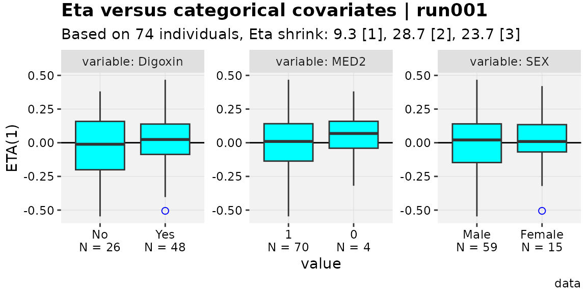
Another way this cross-compatibility is maintained is via custom themes. There may be xpose users concerned about adopting xpose.xtras because with the new plot elements they would have to declare new aesthetic defaults. Conveniently, the xp_xtra theme is derived in a way such that aesthetics for defined plot elements are re-used for similar new elements, meaning there is less (if any) updates needed to use a custom theme beyond using something like the following.

favorite_theme <- xpose::theme_xp_xpose4() # stand-in for "custom" theme

eta_vs_catcov(w_levels,etavar=ETA1, quiet=TRUE)

eta_vs_catcov(w_levels,etavar=ETA1, quiet=TRUE, xp_theme = favorite_theme)

Note that worked even though boxplot_fill is not defined in the xpose::theme_xp_xpose4(). To update an existing theme object to one for the extension package (instead of using the old theme in the xp_theme argument), simply use updated_theme <- xp_xtra_theme(old_theme).

Convenience

xpose has a collection of getter and setter functions to interact with parts of an xpose_data object, but these tend to be lower level and not exported. To add this convenience and make it user-friendly, a few functions have been added.

Properties from a model summary can now be pulled without using xpose::get_summary().

pheno_final %>% get_shk()
#> [1] 20.1 11.6
pheno_final %>% get_shk("eps")
#> [1] 19.6
pheno_final %>% get_prop("ofv")
#> [1] "587.918"
pheno_final %>% get_prop("descr")
#> [1] "na"

xpose has certain expectations around how model descriptions are included in model code. At time of writing, it is expected the format is something like “; 2. Description: (text)”. To add some flexibility, users can either use set_prop() to change description directly, or pull it from a more generic scan of the model code comments using desc_from_comments().

pheno_final %>% desc_from_comments() %>% get_prop("descr")
#> [1] "Reparameterized final model"

It can be helpful to add information to the model data that is available elsewhere in the xpose_data object, such as individual objective functions. Currently, those can be added using backfill_iofv(), which is most often used in the context of xpose_set objects. Theoretically more backfill functions can be made available.