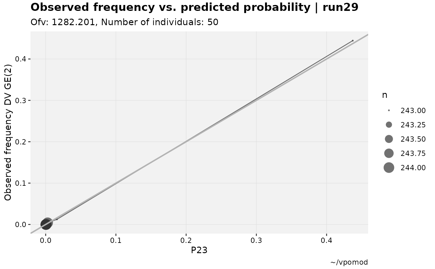
A binned alternative to catdv_vs_dvprobs(). The probability column
associated with cutpoint is split into bins equally-sized groups,
from lowest to highest predicted probability, and for each bin the
observed proportion of the categorical DV meeting the cutpoint
condition is calculated (i.e. the m/M observations in that bin with
the target value).
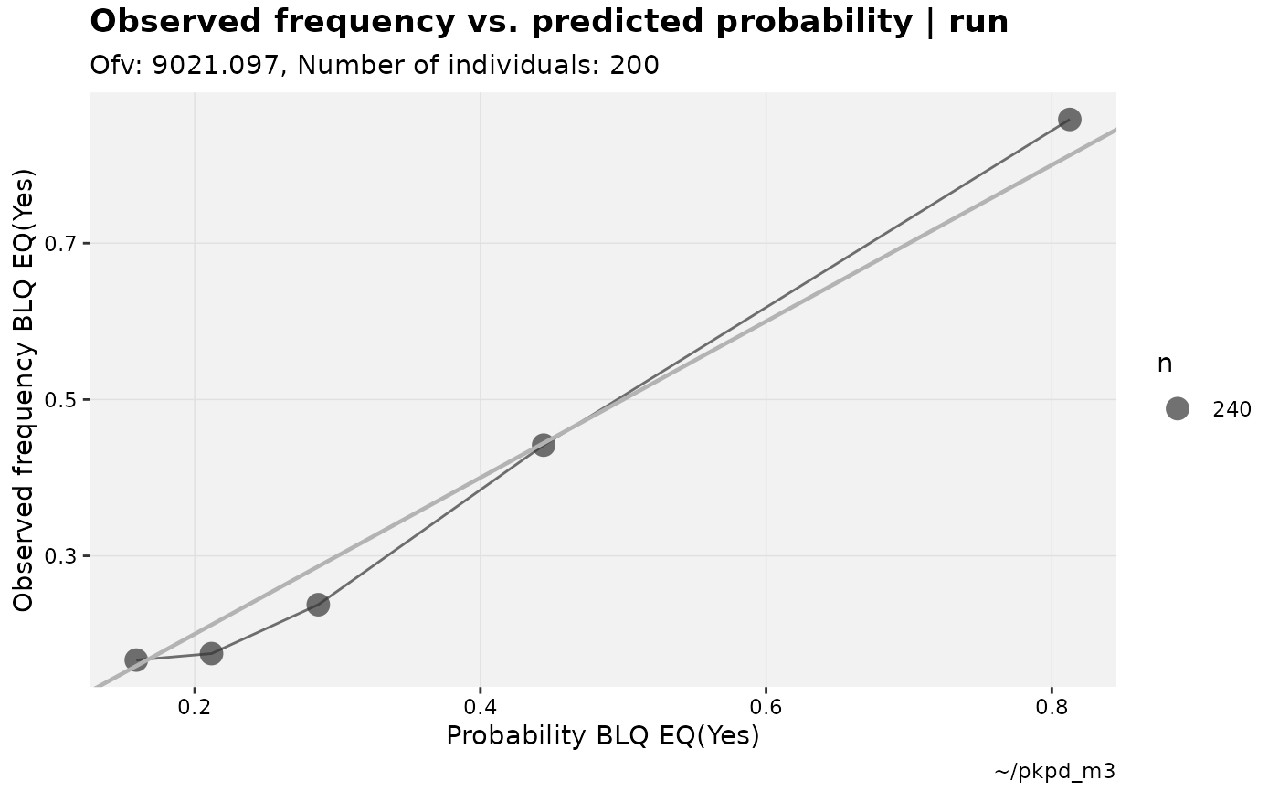
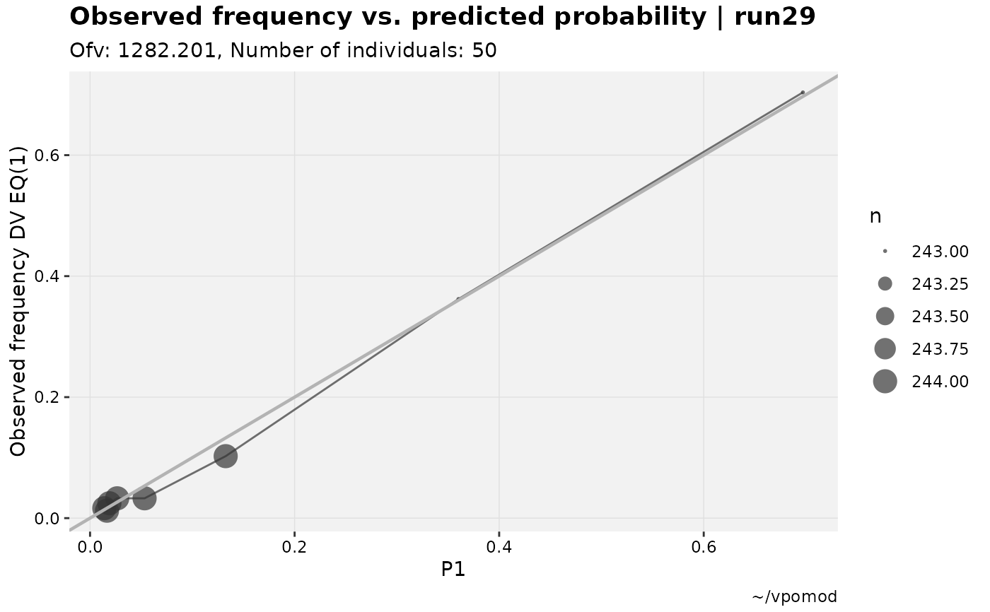
For a well-specified model, the mean predicted probability of a bin
should be close to the bin's observed proportion, so plotted points
are expected to fall around the unity (y = x) line.
Usage
catdv_vs_ipred(
  xpdb,
  mapping = NULL,
  cutpoint = 1,
  bins = 10,
  type = "pl",
  guide = TRUE,
  title = "Observed frequency vs. predicted probability | @run",
  subtitle = "Ofv: @ofv, Number of individuals: @nind",
  caption = "@dir",
  tag = NULL,
  xlab = c("probability", "basic"),
  facets,
  .problem,
  quiet,
  ...
)
Arguments
- xpdb
<
xp_xtras> or <xpose_data> object- mapping
ggplot2style mapping- cutpoint
<
numeric> Of defined probabilities, which one to use in plots.- bins
<
numeric> Number of (roughly) equally-sized bins used to group the probability column, from lowest to highest.- type
String setting the type of plot to be used: line
l, pointp, smoothsand textt, or any combination thereof. Seexpose::xplot_scatter().- guide
Include the unity (
y = x) guide line?- title
Plot title
- subtitle
Plot subtitle
- caption
Plot caption
- tag
Plot tag
- xlab
Either use the typical basic x-axis label (the cutpoint-defined column name) or label it based on the probability/likelihood it is estimating.
- facets
Additional facets
- .problem
Problem number
- quiet
Silence extra debugging output
- ...
Any additional aesthetics.
Examples
# Test M3 model
pkpd_m3 %>%
# Need to ensure var types are set
set_var_types(catdv=BLQ,dvprobs=LIKE) %>%
# Set probs
set_dv_probs(1, 1~LIKE, .dv_var = BLQ) %>%
# Optional, but useful to set levels
set_var_levels(1, BLQ = lvl_bin()) %>%
# Plot with 5 bins
catdv_vs_ipred(bins = 5)
 # Test categorical model
vismo_xpdb <- vismo_pomod %>%
set_var_types(.problem=1, catdv=DV, dvprobs=matches("^P\\d+$")) %>%
set_dv_probs(.problem=1, 0~P0,1~P1,ge(2)~P23)
# Various cutpoints and bin counts
vismo_xpdb %>%
catdv_vs_ipred(bins = 8, xlab = "basic")
# Test categorical model
vismo_xpdb <- vismo_pomod %>%
set_var_types(.problem=1, catdv=DV, dvprobs=matches("^P\\d+$")) %>%
set_dv_probs(.problem=1, 0~P0,1~P1,ge(2)~P23)
# Various cutpoints and bin counts
vismo_xpdb %>%
catdv_vs_ipred(bins = 8, xlab = "basic")
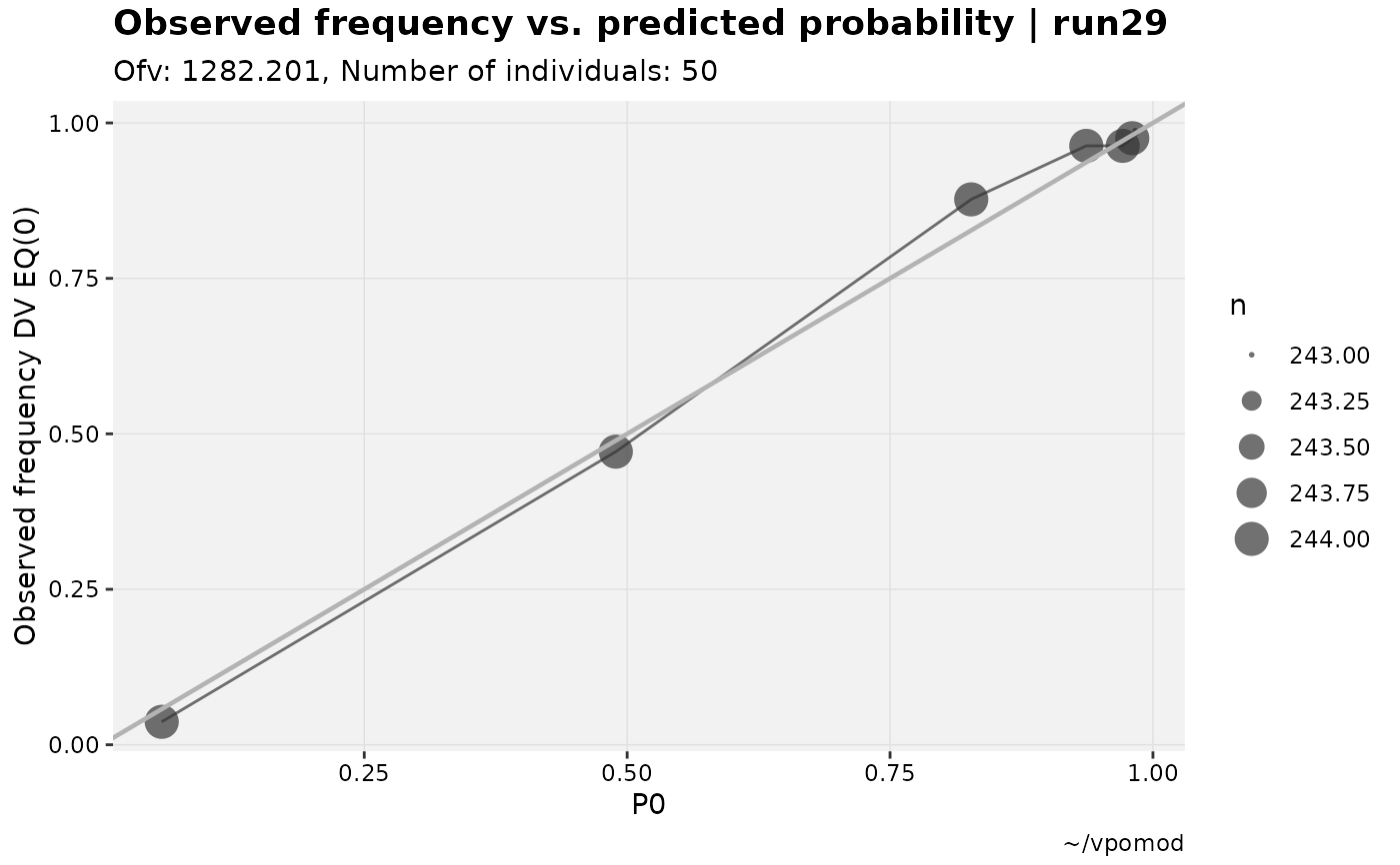 vismo_xpdb %>%
catdv_vs_ipred(cutpoint = 2, bins = 8, xlab = "basic")
vismo_xpdb %>%
catdv_vs_ipred(cutpoint = 2, bins = 8, xlab = "basic")
 vismo_xpdb %>%
catdv_vs_ipred(cutpoint = 3, bins = 8, xlab = "basic")
vismo_xpdb %>%
catdv_vs_ipred(cutpoint = 3, bins = 8, xlab = "basic")