
Parameter Associations: Omega CVs and Covariate Effects
Source:vignettes/articles/parameter-associations.Rmd
parameter-associations.RmdWhy declare anything at all?
A fitted NONMEM (or nlmixr2) model doesn’t carry an
explicit record of why a THETA is where it is.
xpose can read the numbers back out, but it has no way to
know that OMEGA(3,3) is log-normal on CL, or
that THETA(7) is an allometric exponent on
CLCR, rather than something else entirely. Most of the time
that doesn’t matter – get_prm() already assumes log-normal,
which covers the common case – but the moment a model deviates from that
(a logit-transformed variability term, a Box-Cox covariate effect, a
piecewise “hockey-stick” model), xpose has nothing to fall
back on.
xpose.xtras gives you a way to say the quiet part out
loud, once, and have it flow through into reporting:
- [
add_prm_association()] links a structural parameter to the omega driving its between-subject variability, so [get_prm()] can report a meaningful CV% even when the relationship isn’t plain log-normal. - [
add_cov_association()] links a structural parameter to a covariate, so [prm_cov()]/[cov_forest()] can report and plot the covariate’s effect as a ratio to the parameter’s typical value.
The two are deliberately parallel: the same formula-based declaration
style (LHS ~ fun(...)), the same two-stage
validate-then-store behavior, and the same “redeclare to replace”
semantics. This article covers both, plus [mutate_prm()],
the escape hatch for when a parameter isn’t on the scale either
mechanism assumes.
Omega associations and CV%
By default, [get_prm()] treats every diagonal omega as
log-normal and reports CV% accordingly:
pheno_base %>%
  get_prm(quiet = TRUE) %>%
  select(type, name, label, value, cv)
#> # A tibble: 8 × 5
#>   type  name       label      value      cv
#>   <chr> <chr>      <chr>    <num:3> <num:3>
#> 1 the   THETA1     "CL"      0.0068    NA
#> 2 the   THETA2     "V"       1.4       NA
#> 3 the   THETA3     "RUVADD"  2.86      NA
#> 4 the   THETA4     "RUVPRO"  0         NA
#> 5 ome   OMEGA(1,1) "IIVCL"   0.489     52.0
#> 6 ome   OMEGA(2,1) ""        0.998     NA
#> 7 ome   OMEGA(2,2) "IIVV"    0.393     40.9
#> 8 sig   SIGMA(1,1) ""        1         NA
IIVCL and IIVV get a cv
column; the off-diagonal and fixed-effect rows don’t (CV% is only
defined for a diagonal random effect acting on a specific structural
parameter). This is already the CV% you’d get by hand from a log-normal
assumption – add_prm_association() becomes useful the
moment that assumption is wrong for a given parameter.
Say CL was actually fit as logit-normal instead (purely
for illustration – it wasn’t, in this model). Declaring that changes
only the cv column; nothing else about the fit or the table
shape changes:
pheno_base %>%
  add_prm_association(CL ~ logit(IIVCL)) %>%
  get_prm(quiet = TRUE) %>%
  select(type, name, label, value, cv)
#> # A tibble: 8 × 5
#>   type  name       label      value      cv
#>   <chr> <chr>      <chr>    <num:3> <num:3>
#> 1 the   THETA1     "CL"      0.0068    NA
#> 2 the   THETA2     "V"       1.4       NA
#> 3 the   THETA3     "RUVADD"  2.86      NA
#> 4 the   THETA4     "RUVPRO"  0         NA
#> 5 ome   OMEGA(1,1) "IIVCL"   0.489     51.3
#> 6 ome   OMEGA(2,1) ""        0.998     NA
#> 7 ome   OMEGA(2,2) "IIVV"    0.393     40.9
#> 8 sig   SIGMA(1,1) ""        1         NA
#> # Parameter table includes the following associations:
#> CL~logit(IIVCL)
Built-in distributions cover the common cases: log (the
default, made explicit), logexp (log(1+X)),
logit, arcsin, and nmboxcox
(Box-Cox, needs a lambda):
pheno_base %>%
  add_prm_association(V ~ nmboxcox(IIVV, lambda = 0.5)) %>%
  get_prm(quiet = TRUE) %>%
  select(name, label, value, cv)
#> # A tibble: 8 × 4
#>   name       label      value      cv
#>   <chr>      <chr>    <num:3> <num:3>
#> 1 THETA1     "CL"      0.0068    NA
#> 2 THETA2     "V"       1.4       NA
#> 3 THETA3     "RUVADD"  2.86      NA
#> 4 THETA4     "RUVPRO"  0         NA
#> 5 OMEGA(1,1) "IIVCL"   0.489     52.0
#> 6 OMEGA(2,1) ""        0.998     NA
#> 7 OMEGA(2,2) "IIVV"    0.393     38.3
#> 8 SIGMA(1,1) ""        1         NA
#> # Parameter table includes the following associations:
#> V~nmboxcox(IIVV)
For anything else, custom() takes a
qdist/pdist pair (the transform and its
inverse):
pheno_base %>%
  add_prm_association(V ~ custom(IIVV, qdist = function(x) log(0.001 + x), pdist = function(x) exp(x) - 0.001)) %>%
  get_prm(quiet = TRUE) %>%
  select(name, label, value, cv)
#> # A tibble: 8 × 4
#>   name       label      value      cv
#>   <chr>      <chr>    <num:3> <num:3>
#> 1 THETA1     "CL"      0.0068    NA
#> 2 THETA2     "V"       1.4       NA
#> 3 THETA3     "RUVADD"  2.86      NA
#> 4 THETA4     "RUVPRO"  0         NA
#> 5 OMEGA(1,1) "IIVCL"   0.489     52.0
#> 6 OMEGA(2,1) ""        0.998     NA
#> 7 OMEGA(2,2) "IIVV"    0.393     41.0
#> 8 SIGMA(1,1) ""        1         NA
#> # Parameter table includes the following associations:
#> V~custom(IIVV)
Redeclaring an association for the same parameter replaces it;
drop_prm_association() removes it entirely (falling back to
the log-normal default):
pheno_base %>%
  add_prm_association(CL ~ logit(IIVCL)) %>%
  drop_prm_association(CL) %>%
  get_prm(quiet = TRUE) %>%
  select(name, label, value, cv)
#> # A tibble: 8 × 4
#>   name       label      value      cv
#>   <chr>      <chr>    <num:3> <num:3>
#> 1 THETA1     "CL"      0.0068    NA
#> 2 THETA2     "V"       1.4       NA
#> 3 THETA3     "RUVADD"  2.86      NA
#> 4 THETA4     "RUVPRO"  0         NA
#> 5 OMEGA(1,1) "IIVCL"   0.489     52.0
#> 6 OMEGA(2,1) ""        0.998     NA
#> 7 OMEGA(2,2) "IIVV"    0.393     40.9
#> 8 SIGMA(1,1) ""        1         NA
One important caveat: the CV% calculation assumes
the fixed-effect value is on its natural, untransformed scale.
If CL were actually fitted on the logit scale itself (not
just related to a logit-normal omega), the reported value
would need converting back first – see Rescaling with
mutate_prm() below.
Covariate associations and forest plots
The same idea, for covariates instead of omegas. xpdb_x
already has a real covariate effect in it – THETA7, labeled
“CRCL on CL”:
xpdb_x %>%
  get_prm(.problem = 1, quiet = TRUE) %>%
  select(type, name, label, value, se)
#> # A tibble: 11 × 5
#>    type  name       label           value       se
#>    <chr> <chr>      <chr>         <num:3>  <num:3>
#>  1 the   THETA1     "TVCL"       26.3      0.891
#>  2 the   THETA2     "TVV"         1.35     0.0438
#>  3 the   THETA3     "TVKA"        4.2      0.809
#>  4 the   THETA4     "LAG"         0.208    0.0157
#>  5 the   THETA5     "Prop. Err"   0.205    0.0224
#>  6 the   THETA6     "Add. Err"    0.0106   0.00366
#>  7 the   THETA7     "CRCL on CL"  0.00717  0.0017
#>  8 ome   OMEGA(1,1) "IIV CL"      0.27     0.0233
#>  9 ome   OMEGA(2,2) "IIV V"       0.195    0.032
#> 10 ome   OMEGA(3,3) "IIV KA"      1.38     0.202
#> 11 sig   SIGMA(1,1) ""            1       NA
add_cov_association() describes how a covariate affects
a structural parameter, as a ratio to that parameter’s typical value
(always 1 at a declared reference value/level):
xpdb_x %>%
  add_cov_association(TVCL ~ linear(CLCR, THETA7, ref = 64)) %>%
  prm_cov()
#> # A tibble: 3 × 10
#>   param covariate covtype level value is_ref effect ci_low ci_high ci_method
#>   <chr> <chr>     <chr>   <chr> <chr> <lgl>   <dbl>  <dbl>   <dbl> <chr>
#> 1 TVCL  CLCR      cont    low   40    FALSE   0.828  0.747   0.913 simulation
#> 2 TVCL  CLCR      cont    ref   64    TRUE    1      1       1     simulation
#> 3 TVCL  CLCR      cont    high  102   FALSE   1.27   1.14    1.40  simulation
#> # `effect` is a ratio to the parameter's typical value (1 at the reference
#> covariate value/level); CI via simulation.
ref is always required, explicitly –
there’s no way to infer it safely, since NONMEM control streams often
normalize a covariate against a hardcoded constant that isn’t visible
from the xpdb alone.
Built-in forms
Six built-ins cover the usual covariate models, all constructed so
the effect ratio is exactly 1 at ref
regardless of the theta value:
# power (allometric): (COV/ref)^theta
xpdb_x %>% add_cov_association(TVCL ~ power(CLCR, THETA7, ref = 64)) %>% prm_contcov()
#> # A tibble: 3 × 10
#>   param covariate covtype level value is_ref effect ci_low ci_high ci_method
#> * <chr> <chr>     <chr>   <chr> <chr> <lgl>   <dbl>  <dbl>   <dbl> <chr>
#> 1 TVCL  CLCR      cont    low   40    FALSE   0.997  0.995   0.998 simulation
#> 2 TVCL  CLCR      cont    ref   64    TRUE    1      1       1     simulation
#> 3 TVCL  CLCR      cont    high  102   FALSE   1.00   1.00    1.00  simulation
#> # `effect` is a ratio to the parameter's typical value (1 at the reference
#> covariate value/level); CI via simulation.

# exponential: exp(theta*(COV-ref))
xpdb_x %>% add_cov_association(TVCL ~ exponential(CLCR, THETA7, ref = 64)) %>% prm_contcov()
#> # A tibble: 3 × 10
#>   param covariate covtype level value is_ref effect ci_low ci_high ci_method
#> * <chr> <chr>     <chr>   <chr> <chr> <lgl>   <dbl>  <dbl>   <dbl> <chr>
#> 1 TVCL  CLCR      cont    low   40    FALSE   0.842  0.776   0.917 simulation
#> 2 TVCL  CLCR      cont    ref   64    TRUE    1      1       1     simulation
#> 3 TVCL  CLCR      cont    high  102   FALSE   1.31   1.15    1.49  simulation
#> # `effect` is a ratio to the parameter's typical value (1 at the reference
#> covariate value/level); CI via simulation.

# additive: (theta+COV)/(theta+ref) -- an uncommon but simple par = theta + cov model
xpdb_x %>% add_cov_association(TVCL ~ additive(CLCR, THETA7, ref = 64)) %>% prm_contcov()
#> # A tibble: 3 × 10
#>   param covariate covtype level value is_ref effect ci_low ci_high ci_method
#> * <chr> <chr>     <chr>   <chr> <chr> <lgl>   <dbl>  <dbl>   <dbl> <chr>
#> 1 TVCL  CLCR      cont    low   40    FALSE   0.625  0.625   0.625 simulation
#> 2 TVCL  CLCR      cont    ref   64    TRUE    1      1       1     simulation
#> 3 TVCL  CLCR      cont    high  102   FALSE   1.59   1.59    1.59  simulation
#> # `effect` is a ratio to the parameter's typical value (1 at the reference
#> covariate value/level); CI via simulation.

# hockey-stick (PsN-style): different slope above/below ref (which doubles as the
# breakpoint by default; see `brk=` to separate them)
xpdb_x %>% add_cov_association(TVCL ~ hockey(CLCR, THETA7, THETA4, ref = 64)) %>% prm_contcov()
#> # A tibble: 3 × 10
#>   param covariate covtype level value is_ref effect ci_low ci_high ci_method
#> * <chr> <chr>     <chr>   <chr> <chr> <lgl>   <dbl>  <dbl>   <dbl> <chr>
#> 1 TVCL  CLCR      cont    low   40    FALSE   0.828  0.747   0.913 simulation
#> 2 TVCL  CLCR      cont    ref   64    TRUE    1      1       1     simulation
#> 3 TVCL  CLCR      cont    high  102   FALSE   8.90   7.68   10.1   simulation
#> # `effect` is a ratio to the parameter's typical value (1 at the reference
#> covariate value/level); CI via simulation.

# catshift: one theta per non-reference categorical level
xpdb_x %>% add_cov_association(TVCL ~ catshift(SEX, THETA4, ref = 1)) %>% prm_catcov()
#> # A tibble: 2 × 10
#>   param covariate covtype level value is_ref effect ci_low ci_high ci_method
#> * <chr> <chr>     <chr>   <chr> <chr> <lgl>   <dbl>  <dbl>   <dbl> <chr>
#> 1 TVCL  SEX       cat     1     1     TRUE     1      1       1    simulation
#> 2 TVCL  SEX       cat     2     2     FALSE    1.21   1.18    1.24 simulation
#> # `effect` is a ratio to the parameter's typical value (1 at the reference
#> covariate value/level); CI via simulation.
Note how differently power and linear read
the same THETA7: a power exponent of
0.007 barely moves the ratio across any realistic
CLCR range, while the same number as a linear slope gives a
substantial swing. Picking the right built-in for how the
covariate actually enters the model matters – the computation
can’t tell the two apart for you, and a mismatched builtin produces a
numerically valid but silently wrong ratio. When none of the built-ins
fit, custom() takes a fun(cov, ref, theta),
validated at declaration time to confirm
fun(ref, ref, theta) == 1 for a few probe thetas:
xpdb_x %>%
  add_cov_association(
    TVCL ~ custom(CLCR, THETA7, ref = 64, fun = function(cov, ref, theta) (cov / ref)^theta)
  ) %>%
  prm_contcov()
#> # A tibble: 3 × 10
#>   param covariate covtype level value is_ref effect ci_low ci_high ci_method
#> * <chr> <chr>     <chr>   <chr> <chr> <lgl>   <dbl>  <dbl>   <dbl> <chr>
#> 1 TVCL  CLCR      cont    low   40    FALSE   0.997  0.995   0.998 simulation
#> 2 TVCL  CLCR      cont    ref   64    TRUE    1      1       1     simulation
#> 3 TVCL  CLCR      cont    high  102   FALSE   1.00   1.00    1.00  simulation
#> # `effect` is a ratio to the parameter's typical value (1 at the reference
#> covariate value/level); CI via simulation.
drop_cov_association() removes a declared (parameter,
covariate) pair, the same way drop_prm_association() works
for omegas:
xpdb_x %>%
  add_cov_association(TVCL ~ linear(CLCR, THETA7, ref = 64)) %>%
  drop_cov_association(TVCL ~ CLCR) %>%
  prm_cov()
#> # A tibble: 0 × 10
#> # ℹ 10 variables: param <chr>, covariate <chr>, covtype <chr>, level <chr>,
#> #   value <chr>, is_ref <lgl>, effect <dbl>, ci_low <dbl>, ci_high <dbl>,
#> #   ci_method <chr>
prm_cov() output
prm_contcov()/prm_catcov()/prm_cov()
all return the same shape: one row per (parameter, covariate, evaluation
point), with
effect/ci_low/ci_high as ratios
to the typical value, and an is_ref flag for the
(uninformative, always-1) reference row:
xpdb_x %>%
  add_cov_association(
    TVCL ~ linear(CLCR, THETA7, ref = 64),
    TVCL ~ catshift(SEX, THETA4, ref = 1)
  ) %>%
  prm_cov()
#> # A tibble: 5 × 10
#>   param covariate covtype level value is_ref effect ci_low ci_high ci_method
#>   <chr> <chr>     <chr>   <chr> <chr> <lgl>   <dbl>  <dbl>   <dbl> <chr>
#> 1 TVCL  CLCR      cont    low   40    FALSE   0.828  0.747   0.913 simulation
#> 2 TVCL  CLCR      cont    ref   64    TRUE    1      1       1     simulation
#> 3 TVCL  CLCR      cont    high  102   FALSE   1.27   1.14    1.40  simulation
#> 4 TVCL  SEX       cat     1     1     TRUE    1      1       1     simulation
#> 5 TVCL  SEX       cat     2     2     FALSE   1.21   1.18    1.24  simulation
#> # `effect` is a ratio to the parameter's typical value (1 at the reference
#> covariate value/level); CI via simulation.
Continuous covariates are evaluated at the 5th/95th percentile of the
observed data (probs=) plus the reference; categorical
covariates at every observed level. The confidence interval comes from
ci_method: "simulation" (default) draws from
N(theta_hat, se) and propagates through the (possibly
nonlinear) effect function; "delta" is a cheaper
first-order analytic approximation.
Plotting: cov_forest()
xpdb_x %>%
  add_cov_association(
    TVCL ~ linear(CLCR, THETA7, ref = 64),
    TVCL ~ catshift(SEX, THETA4, ref = 1)
  ) %>%
  cov_forest()
#> Using data from $prob no.1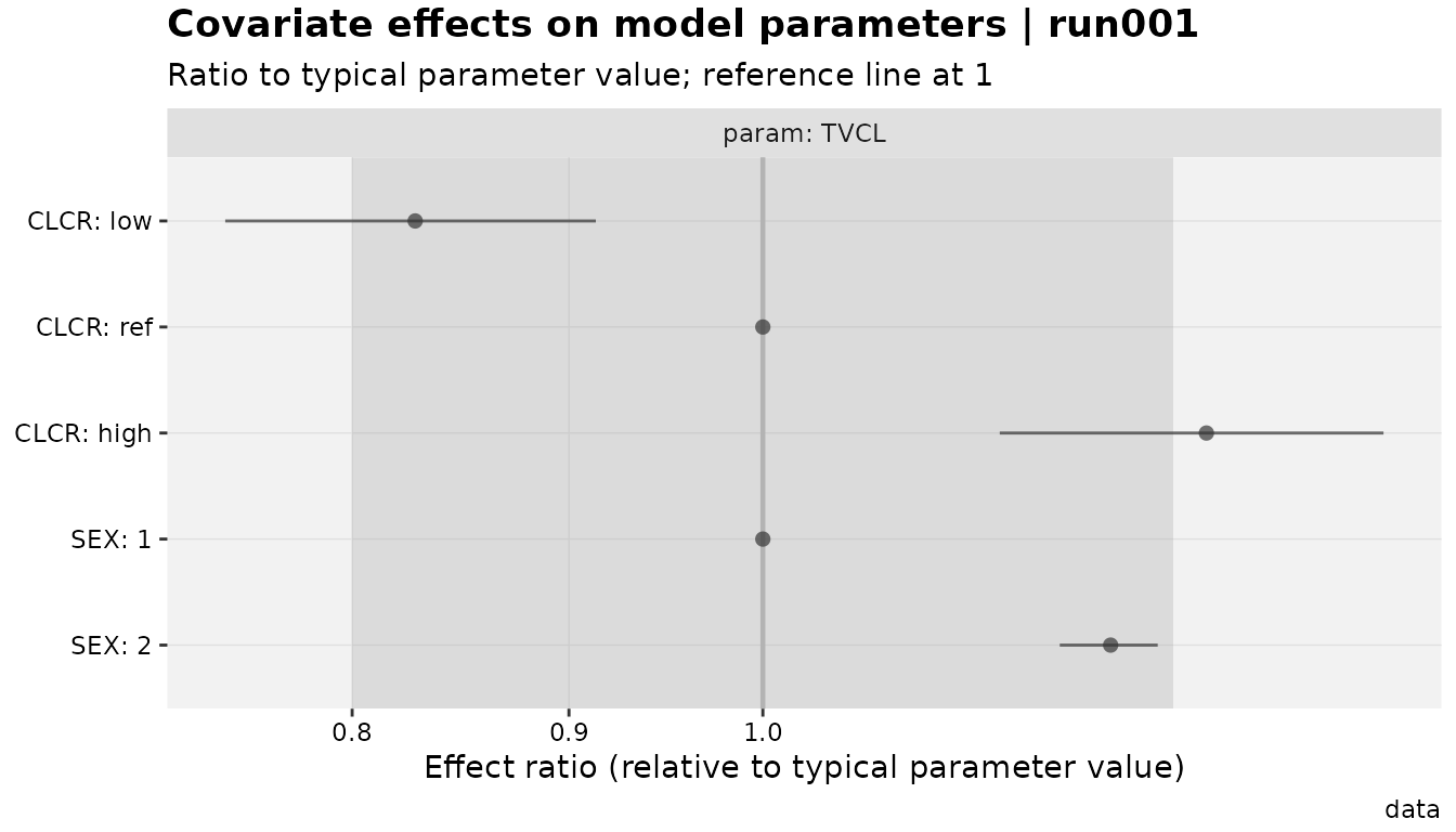
The default view includes a reference line at 1, a
shaded “no relevant effect” band (region=, default
c(0.8, 1.25), a common bioequivalence-style convention –
override or drop it with type=), and one row per evaluation
point. show_ref = FALSE drops the uninformative reference
rows; TVCL ~ CLCR (or any param ~ covariate
formula) restricts which declared associations get plotted:
xpdb_x %>%
  add_cov_association(
    TVCL ~ linear(CLCR, THETA7, ref = 64),
    TVCL ~ catshift(SEX, THETA4, ref = 1)
  ) %>%
  cov_forest(TVCL ~ CLCR, show_ref = FALSE, region = c(0.7, 1.43))
#> Using data from $prob no.1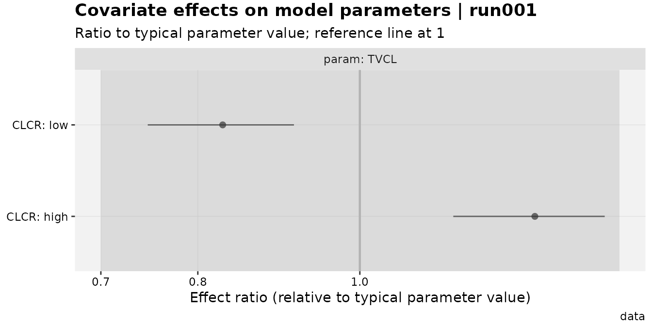
Including "v" in type adds a violin layer
showing the actual simulation draws behind each interval (requires
ci_method = "simulation", the default):
xpdb_x %>%
  add_cov_association(
    TVCL ~ linear(CLCR, THETA7, ref = 64),
    TVCL ~ catshift(SEX, THETA4, ref = 1)
  ) %>%
  cov_forest(type = "pilrv")
#> Using data from $prob no.1
#> Re-fetching data for the violin layer (one row per draw, a different shape than
#> the point/interval data).
#> Using data from $prob no.1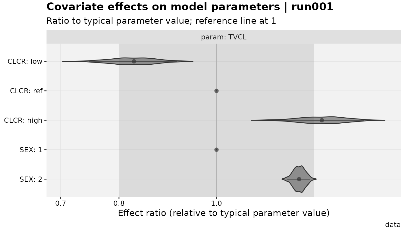
cov_forest() is the covariate-specific wrapper around a
generic, forest-plot-agnostic renderer, [xplot_forest()] –
the same split as
eta_vs_catcov()/xplot_boxplot() elsewhere in
the package. Reaching for xplot_forest() directly is only
useful when plotting something other than a
prm_cov() table.
Rescaling with mutate_prm()
Both association mechanisms assume a specific scale:
add_prm_association() assumes the fixed-effect value is
untransformed (natural units, not logit/log/whatever);
add_cov_association() assumes the chosen builtin’s formula
matches the model code, including how the LHS parameter itself was
parameterized – though notably, the covariate computation never
touches the LHS’s own fitted value, only the covariate-effect
theta, so it’s automatically agnostic to whether the LHS was log- or
identity-parameterized.
When a parameter genuinely needs converting first,
[mutate_prm()] does that in place, updating both the value
and (via simulation) its standard error:
# Say THETA12 in vismo_pomod was fitted on the logit scale, and needs to be
# expressed on the natural (0-1) scale before an association is declared
vismo_pomod %>%
  mutate_prm(THETA12 ~ plogis) %>%
  get_prm(quiet = TRUE) %>%
  filter(name == "THETA12") %>%
  select(name, label, value, se)
#> Warning: [$prob no.1, subprob no.1, lce] $SIGMA labels did not match the number
#> of SIGMAs in the `.ext` file.
#> Warning: Shrinkage missing for sigma estimates, if any are modeled. Using NA in this
#> table.
#> # A tibble: 1 × 4
#>   name    label                                                    value      se
#>   <chr>   <chr>                                                   <num:> <num:3>
#> 1 THETA12 THETA(12) ; B1: baseline of LOGIT(P(AE>=1)); final est… 0.0157 0.00302
This is the same recommendation
[add_prm_association()]’s own documentation already carries
for the logit/Box-Cox omega case – reach for mutate_prm()
first, then declare the association on the now-natural-scale value.
Session info
sessionInfo()
#> R version 4.6.1 (2026-06-24)
#> Platform: x86_64-pc-linux-gnu
#> Running under: Ubuntu 24.04.4 LTS
#>
#> Matrix products: default
#> BLAS:   /usr/lib/x86_64-linux-gnu/openblas-pthread/libblas.so.3
#> LAPACK: /usr/lib/x86_64-linux-gnu/openblas-pthread/libopenblasp-r0.3.26.so;  LAPACK version 3.12.0
#>
#> locale:
#>  [1] LC_CTYPE=C.UTF-8       LC_NUMERIC=C           LC_TIME=C.UTF-8
#>  [4] LC_COLLATE=C.UTF-8     LC_MONETARY=C.UTF-8    LC_MESSAGES=C.UTF-8
#>  [7] LC_PAPER=C.UTF-8       LC_NAME=C              LC_ADDRESS=C
#> [10] LC_TELEPHONE=C         LC_MEASUREMENT=C.UTF-8 LC_IDENTIFICATION=C
#>
#> time zone: UTC
#> tzcode source: system (glibc)
#>
#> attached base packages:
#> [1] stats     graphics  grDevices utils     datasets  methods   base
#>
#> other attached packages:
#> [1] xpose.xtras_0.2.2 xpose_0.4.23      ggplot2_4.0.3     dplyr_1.2.1
#>
#> loaded via a namespace (and not attached):
#>  [1] utf8_1.2.6         sass_0.4.10        generics_0.1.4     tidyr_1.3.2
#>  [5] stringi_1.8.9      hms_1.1.4          digest_0.6.39      magrittr_2.0.5
#>  [9] evaluate_1.0.5     grid_4.6.1         RColorBrewer_1.1-3 fastmap_1.2.0
#> [13] jsonlite_2.0.0     backports_1.5.1    purrr_1.2.2        scales_1.4.0
#> [17] tweenr_2.0.3       textshaping_1.0.5  jquerylib_0.1.4    cli_3.6.6
#> [21] rlang_1.3.0        polyclip_1.10-7    withr_3.0.3        cachem_1.1.0
#> [25] yaml_2.3.12        otel_0.2.0         tools_4.6.1        tzdb_0.5.0
#> [29] checkmate_2.3.4    forcats_1.0.1      vctrs_0.7.3        R6_2.6.1
#> [33] lifecycle_1.0.5    stringr_1.6.0      fs_2.1.0           htmlwidgets_1.6.4
#> [37] MASS_7.3-65        ragg_1.5.2         pkgconfig_2.0.3    desc_1.4.3
#> [41] pkgdown_2.2.1      pillar_1.11.1      bslib_0.12.0       gtable_0.3.6
#> [45] glue_1.8.1         pmxcv_0.0.2        ggforce_0.5.0      systemfonts_1.3.2
#> [49] xfun_0.60          tibble_3.3.1       tidyselect_1.2.1   knitr_1.51
#> [53] farver_2.1.2       htmltools_0.5.9    rmarkdown_2.31     readr_2.2.0
#> [57] compiler_4.6.1     S7_0.2.2